Educational disclaimer. The algorithm is described by analogy; the papers cited under each claim carry the scientific detail. Service limits, free tiers and hardware names are snapshots from the day this was written and will drift. Treat the Kipu Quantum Hub and the linked papers as the single sources of truth.
1. Triage the fit
Three questions that decide whether a problem maps onto quantum optimization at all.
2. Read the method
Adiabatic evolution, the counterdiabatic shortcut, and the bias-field loop behind Miray and Iskay.
3. Judge the evidence
What the 156-qubit end-to-end benchmark preprint claims, what it does not, and the two numbers worth asking for.
What is quantum optimization?
Quantum optimization is the act or process of finding the absolute highest or lowest value of a function under specific rules, carried out by mapping that function into quantum states and using phenomena such as superposition and tunneling to navigate the solution landscape. The first half of that sentence is ordinary mathematical optimization, the discipline behind every scheduling tool and every portfolio model your organization already runs. The second half is the only part that is new: the search itself is performed by a physical quantum system rather than by a classical processor stepping through candidate answers.
That framing tells you where the quantum part can help. It does not invent your objective, it does not know your business rules, and it does not replace the classical software around it. It is a specialist search engine you hand a finished mathematical model, and it hands back ranked candidate answers.
quan·tum op·ti·mi·za·tion
/ˈkwɒn.təm ˌɒp.tɪ.maɪˈzeɪ.ʃən/noun
- 1
act or process of finding the absolute highest or lowest values of a function under specific rules.
- 2
a method that maps complex math problems into quantum states, using phenomena like superposition and tunneling to navigate tricky solution landscapes.
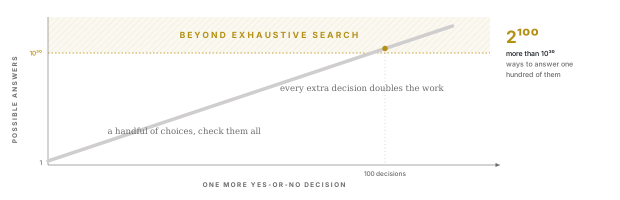
The problems in scope are combinatorial: a finite set of discrete choices whose combinations multiply faster than any machine can enumerate. Pick a subset of assets, assign crews to shifts, route a truck across segments. Classical exact solvers eventually hit that wall and stop being able to guarantee anything; classical heuristics stay useful by searching cleverly rather than exhaustively. Quantum optimization joins that second group. It is a heuristic, and it competes with other heuristics on measured results, not on a proof.
Does your problem fit? Three questions
Before anyone talks about hardware, a problem has to survive a triage. Three questions decide it, and each one has a standard workaround if the answer is no.
Does your problem fit? Three questions.
Is the core decision binary?
select / don't select · assign / don't assign · route via A or not
Is there one number to optimize?
cost · time · energy · risk
Can the rules become penalties?
“exactly 50 assets” · “no crew works two shifts back to back”
Answer all three to get a verdict.
Is the core decision binary? Today's quantum optimizers work on yes/no variables, each taking the value 0 or 1. Select or don't select. Assign or don't assign. Route via A or not. Continuous quantities are not disqualifying, because they can usually be bucketed into a set of binary choices, but the buckets cost variables, so the reshaping is a real design decision rather than a formality.
Is there one number to optimize? Cost, time, energy, risk. The solver ranks candidate answers against a single figure of merit. If you have three objectives, you have to choose weights between them, and that is a business decision made by people, not a mathematical one the solver can make for you. Better to settle it consciously and up front than to discover it hidden in a formula later.
Can the rules become penalties? Every constraint has to be re-expressed as a cost added to any solution that breaks it. "Exactly fifty assets in the portfolio" becomes a term that grows when the count is wrong. "No crew works two shifts back to back" becomes a term that fires when the pattern appears. A hard physical limit is enforced by making its penalty large enough that no sensible answer ever pays it.
Three yes answers and the problem maps onto quantum optimization. A no names the reshaping step rather than ending the exercise: bucket the continuous quantities, fix the weights between the competing objectives, write the constraints as penalties. A problem that still sits outside after that is worth recording as outside, together with the reason it does.
How do you write it down for the solver?
The translation is mechanical once the triage is passed. Five steps:
- Turn every yes/no decision into one binary variable.
- Give each variable a coefficient: the cost or the gain of choosing it.
- Where two decisions interact, a risky pair of assets or two flights on the same corridor, join them with a term. Where three or more interact, join those too.
- Write each rule as a penalty term, as in the triage above.
- Add the whole thing up. You now have one function over all the bits.
In the jargon it is a QUBO when interactions are pairwise only, and a HUBO, higher-order unconstrained binary optimization, when triples and higher appear. Kipu's solvers take HUBOs natively, so a genuinely three-body risk term does not have to be flattened into pairs first.
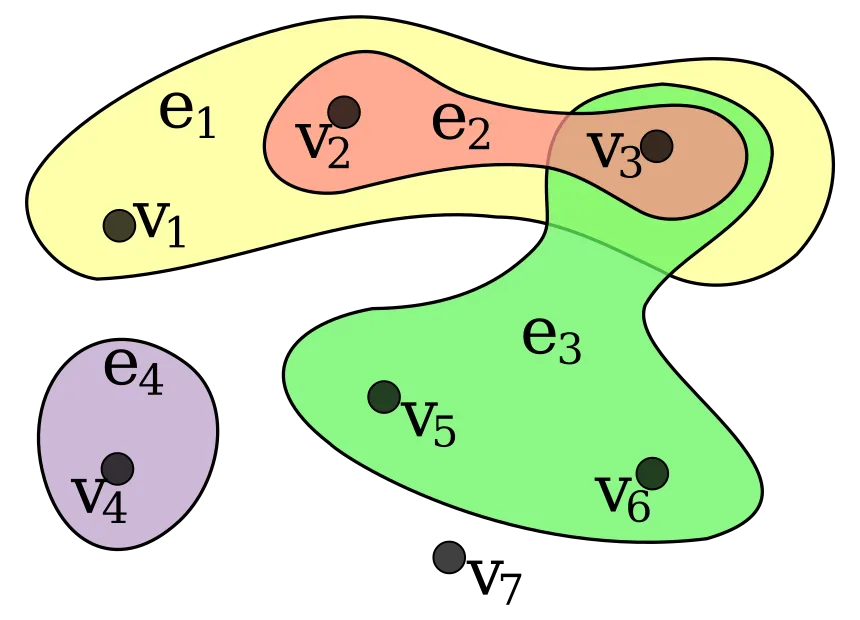
Native HUBO expressiveness is more than a modeling convenience. A business rule with three or more decisions interacting, kept as one higher-order term instead of flattened into pairwise penalty terms, uses less of the quantum resource each solve consumes. A published study from Lufthansa Industry Solutions (Koch, Panahiyan, Mukherjee and Doetsch, with Jaksch) encoded constraints this way instead of as QUBO penalties and reported at least 89.6 percent fewer CNOT gates on every tested instance, across gate assignment, graph coloring and integer programming (arXiv:2511.17545, EPJ Quantum Technology 2026). On current NISQ devices, CNOT gates need to be optimized: fewer of them for the same problem is a smaller strain on the hardware. Since each operation adds to an error, this noise dictates whether a solution is found, and how many shots we need to measure it. Less is more in this case. And the advantage compounds, smaller circuits mean not only reduced error rates, but faster execution times, too.
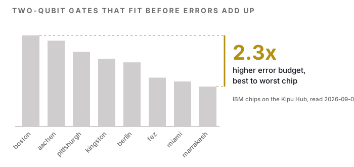
There is a number behind that, and you can read it off the hardware. A chip's median two-qubit error rate and its coherence time together say how many two-qubit gates fit into a circuit before the errors add up to order one and the answer drowns. Take whichever limit binds first, one over the median two-qubit error rate or the coherence time divided by the gate time, min(1/p_2q, T2/t_2q). Read on 2026-09-07 across the eight IBM chips bookable on the Kipu Quantum Hub, that budget ran from about 680 gates on boston down to about 298 on marrakesh, a factor of 2.3 between chips you could queue on the same afternoon. The error rate is what binds on every one of them; coherence never runs out first. Boston's calibration record was a day older than the rest, which is the ordinary state of these numbers: each chip is recalibrated on its own schedule and the values drift. So the chip you name when you submit moves your circuit budget by more than a hardware generation's headline improvement usually does.
One candidate solution is therefore one string of bits, and the whole search is a walk over those strings. The value of the function at each string is its cost, and the answer you want is the string with the lowest cost. Picture that as a landscape with valleys: the deepest valley is the optimum, and every other valley is a spot where flipping any single decision makes things worse, which is exactly where cheap classical descent gets stuck.
Real landscapes are rugged. That ruggedness is the reason this problem class stays hard no matter how large your compute cluster is, and it is the reason a physically different way of searching is worth testing.
Protein folding, as an example of the encoding
Given a protein's amino acid sequence, what is its three-dimensional structure? Placing the sequence on a lattice makes this a combinatorial problem: monomers must sit on adjacent lattice sites without overlapping, and the number of configurations grows combinatorially with sequence length. Most configurations are invalid, and validity is a lattice constraint, so it enters the model as a penalty.
The encoding uses two families of terms, one for the conformation itself and one for contacts between monomers, and produces an Ising Hamiltonian with terms up to three bodies, plus four- and five-body terms in the fuller versions. That is a textbook higher-order problem, and it is why native HUBO support is not a convenience feature. Source: Robert, A., Barkoutsos, P. K., Woerner, S. et al., Resource-efficient quantum algorithm for protein folding, npj Quantum Information 7, 38 (2021).
How does it work?
Kipu's optimizer implements an algorithm called BF-DCQO, bias-field digitized counterdiabatic quantum optimization. The name is a stack of three ideas, and each one is a fix for a specific problem with the idea before it. Read them in order and the whole thing becomes legible without a single equation.
The starting idea: evolve slowly
In adiabatic quantum computing, you start the machine in the easily prepared lowest-energy state of a simple system, then change that system slowly into the one whose lowest-energy state encodes your answer. If the change is slow enough, the system stays in its lowest-energy state throughout, and when you stop, reading the qubits gives you the solution.
Three things follow. In principle any computational problem can be encoded this way, so the approach is universal. The required runtime depends on the smallest energy gap the system passes through on its way, and for hard problems that gap tends to be small, which makes the run long. And a long run needs a machine that holds its quantum state for a long time, which today's hardware does not. Adiabatic evolution is the right intuition and the wrong implementation.
The first fix: take a shortcut
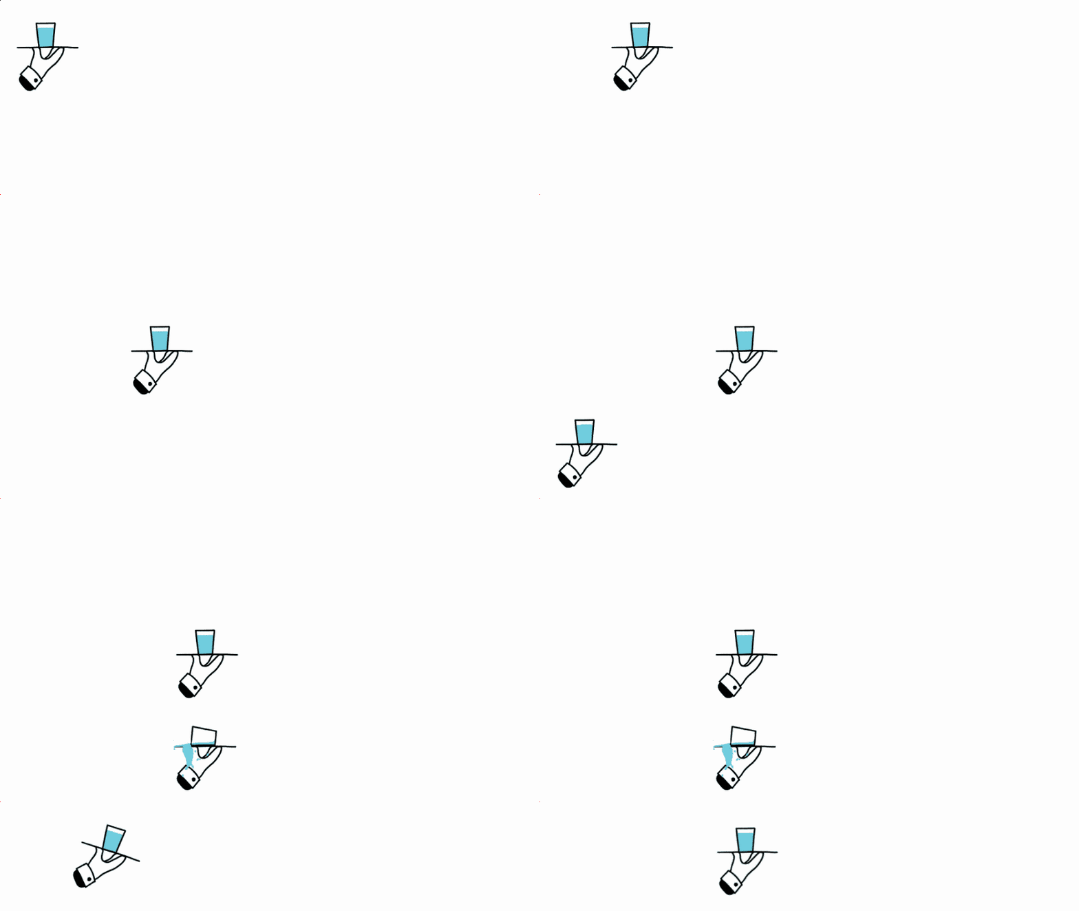
Counterdiabatic protocols let you go fast anyway. Think of carrying a flask of liquid. Tilt it slowly and the surface stays level. Tilt it fast and the liquid sloshes and spills. But tilt it fast while applying a compensating counter-motion, and the surface stays level at speed. The counterdiabatic term is that compensating motion: an extra piece added to the evolution that suppresses the transitions a fast schedule would otherwise cause.
Computing that compensating term exactly requires knowing the answer already, so in practice it is approximated by truncating a series expansion. The approximation is what makes it implementable: a short circuit instead of a long slow sweep, which is precisely what current hardware can run. None of this is new with quantum computers. The counterdiabatic idea predates quantum computing hardware by a decade and a half, developed in the physical chemistry and quantum control literature (Demirplak and Rice 2003, Berry 2009, Takahashi 2013, Sels and Polkovnikov 2017, Claeys et al. 2019).
The second fix: start closer, then iterate
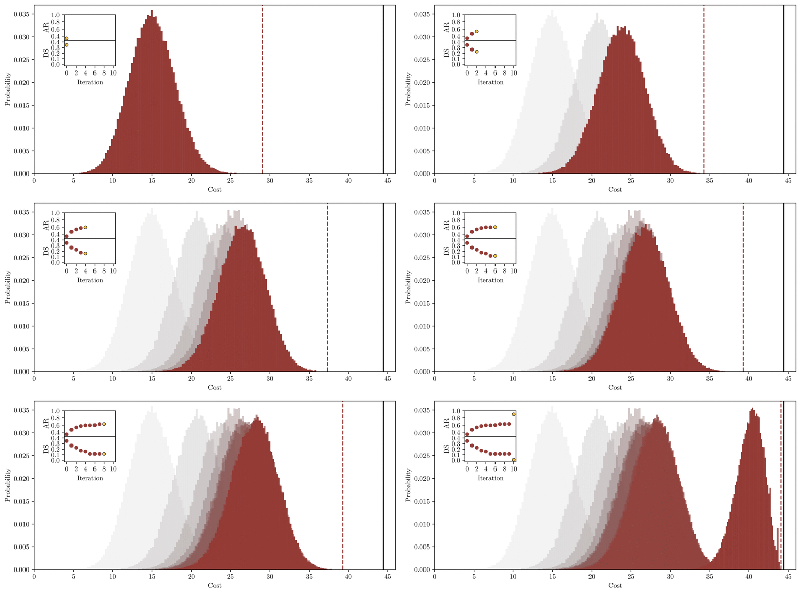
A shortcut from an uninformed starting point still has a long way to go. The bias field is the answer to that. The first run begins with no preference at all: every one of the possible bit strings is equally likely. You run the short circuit a few thousand times, between 1,000 and 10,000 in the published experiments, and each run, called a shot, returns one candidate answer. How long a shot takes is a property of the hardware and not of the algorithm: microseconds on the superconducting processors this solver runs on today, of the order of a second on neutral-atom machines. A few thousand superconducting shots is therefore seconds of quantum time, which is what makes an iterative loop affordable in the first place. The measurement statistics across those shots say something about which decisions tend to be worth making. That information is folded back into the starting point of the next run as a small per-variable bias, so the second run starts nearer the good region than the first did. Then it repeats.
The published experiments use about ten rounds: ten in the Physical Review Research scaling study, eleven in the 156-qubit Communications Physics run, at both 156 and 433 variables. Fewer are needed when the first run is warm-started from a classical solution instead of from no preference at all, and the Hub run shown later on this page uses five. Circuits also get cheaper as the loop proceeds, because a better starting point needs less evolution to finish the job. The loop is what the "BF" stands for.
Keeping noise out of the loop
There is an obvious failure mode in a loop that learns from measurements: on noisy hardware, some of those measurements are corrupted, and a naive average would let the noise steer the next round. BF-DCQO handles this with a CVaR-based update rule. Instead of averaging all shots, it keeps only the best-scoring tail of them, a tunable fraction, and updates the bias field from that tail alone. High-energy shots, which is where noise mostly lands, are discarded before they can influence anything.
The commercial consequence is a cost one. Because the noise handling is part of the update rule and not a mitigation layer wrapped around it, it consumes no additional shots and no additional circuits, and on a machine billed by quantum runtime those are the two things you pay for.
Why this algorithm and not another?
Four properties separate BF-DCQO from the variational quantum algorithms that dominated earlier work on quantum optimization, and they are why it is the engine Kipu productizes. All four are reported in Gómez Cadavid, A. et al., Physical Review Research 7, L022010 (2025) and Romero V., S. et al., Communications Physics 8, 348 (2025); the algorithm itself is described in arXiv:2409.04477.
No classical optimizer sits in the loop tuning circuit parameters, which is what a variational algorithm does and what gives it trainability problems as it scales. Here the measurement statistics update the starting point directly, and the circuit parameters are obtained analytically, so moving to more qubits requires no retraining. Noise robustness comes from the CVaR-based bias field described above; because that sits inside the algorithm rather than in a mitigation layer on top, it costs no additional shots or circuits. And that absence changes the shot budget structurally, not just marginally. A variational method has to be trained before it can be sampled: a classical optimizer spends shots evaluating candidate circuit parameters, and those shots are discarded once it settles, because their only job was to tune the circuit. Only then does sampling for an answer begin. Here there is no training phase, and every shot is simultaneously evidence for the next bias field and a candidate answer in its own right, so nothing is thrown away.
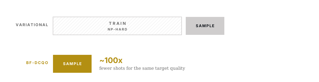
That is why the totals separate by two orders of magnitude in shots, and around ten iterations suffice where variational methods usually need about a hundred. On machines billed by quantum runtime the sampling budget is the bill, which is where that difference is felt.
Circuit size looks like a separate question and turns out to be the same one. Count the gates in a single QAOA layer and it is not an expensive circuit, sometimes cheaper than the counterdiabatic alternative. The catch is what one layer buys you: at a single repetition the prepared state overlaps the actual solution only faintly, and the number of shots you need before that solution appears in your measurements goes as one over that overlap. A cheap circuit you must run a very large number of times is not cheap. Buying more overlap means more layers, which multiplies the depth and enlarges the training problem at the same time.
So the comparison that matters is made at the point where each method actually reaches an answer, not per layer. Measured that way the counterdiabatic route runs shallower and converges more often, which is the same fact as needing about a hundred times fewer shots, seen from the circuit side rather than the budget side.
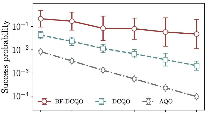
That plot ranks the three methods against each other; it does not forecast absolute performance. Success probability falls off as problems get bigger for all three, and the fitted decay rate is simply slower for BF-DCQO at 0.0840 than for plain digitized counterdiabatic optimization at 0.1283 or adiabatic optimization at 0.1940 (Gómez Cadavid et al. 2025, qubit counts on a log scale). What it establishes is that the bias-field loop earns its keep against its own ancestors. It carries no information about classical solvers.
How does it compare to classical solvers?
Beating your own predecessors is table stakes. The commercially interesting question is how a quantum pipeline does against the classical solvers a company would otherwise buy, measured end to end, on the same problems.
Start with what can and cannot be settled on paper. BF-DCQO is a heuristic, so it carries no a-priori bound on how far a returned answer sits from the optimum. Individual properties can be established analytically, noise robustness among them, and scaling behaviour can be measured across a range of problem sizes, which is what the plot above does. General performance against another heuristic has to be benchmarked empirically. That is not a quantum caveat: simulated annealing carries the same absence of a guarantee, and so does an exact solver like CPLEX the moment it is stopped before it has proved optimality. So an advantage claim is only readable if it names its classical baseline and its metric, and that applies to the numbers below as much as to anyone else's.
A preprint from Kipu Quantum with IBM Research Europe, TU Berlin, the Zuse Institute Berlin and the University of the Basque Country reports exactly that benchmark: an end-to-end evaluation of a hybrid quantum solver for HUBO problems on IBM Heron r3 processors, published as arXiv:2603.13607.
Four things about the setup decide what the result is worth. The problems were made hard on purpose: higher-order binary optimization at sizes reaching 156 qubits, with as many as a thousand three-body terms, and coefficients drawn from heavy-tailed Cauchy distributions rather than a uniform range. The heavy tails are the point, because they produce the badly conditioned landscapes that a friendlier benchmark would avoid.
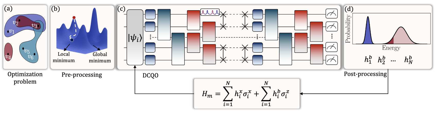
The pipeline is hybrid and says so. Classical preprocessing, then quantum optimization with BF-DCQO, then classical post-processing, with the classical stages counted inside the measured time rather than treated as setup.
The metric is runtime to reach a target solution quality, measured against five classical baselines: memetic tabu search, simulated annealing, parallel tempering, and the QUBO++ solvers EasySolve and ABS3. Time-to-target is the comparison that stays honest, because best-answer-ever rewards whichever solver was given the longest run.
The sampling budgets are uneven by six orders of magnitude, in the classical solvers' favour. Classical sampling runs at gigahertz rates and quantum sampling on today's hardware at kilohertz rates, so the quantum side draws roughly a million times fewer samples per second than the baselines it is being timed against.
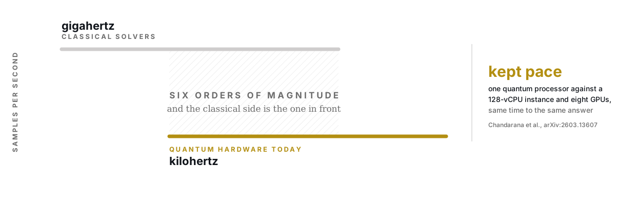
On that footing the hybrid pipeline came out competitive: one quantum processor reached the target quality in comparable time to a 128-vCPU classical instance, and to eight data-centre GPUs, on this problem family (Chandarana, P. et al., arXiv:2603.13607, verified 2026-08-20). An earlier study from the same group reported the complementary result on 156-qubit IBM devices, a faster time-to-approximate-solution than simulated annealing and CPLEX on the hard instances it selected (arXiv:2505.08663, verified 2026-08-20).
Both are preprints rather than peer-reviewed results, and competitive is not better. What they suggest is a trajectory rather than an advantage: a pipeline drawing a million times fewer samples per second already keeps pace on this problem family, which locates the remaining gap in hardware sampling rates rather than in the algorithm. No commercial-scale quantum advantage in combinatorial optimization has been demonstrated in this field, by Kipu or by anyone else, and this benchmark is not one.
Why not just run it once and read the answer?
On an idealized machine running a perfectly slow adiabatic evolution, a single measurement would suffice: the system would end in its lowest-energy state and one readout would give you the answer. In principle, one shot.
Two things break that in practice. The evolution time required is set by the smallest energy gap the system passes through, which for hard problems is small enough to make the run long, and the machine has to hold its quantum state for the whole of it. Neither condition is met by current hardware. So instead of one long perfect run you take many short imperfect ones and learn from the statistics, which is why the shot count is what determines the cost of a run.
Can you try it? Miray on the Kipu Quantum Hub
The algorithm reaches you as a service. Miray Advanced Quantum Optimizer is the BF-DCQO implementation on the Kipu Quantum Hub marketplace, and Iskay is the same solver family delivered as a Qiskit Function for teams working inside IBM's stack. You subscribe to the solver and build the wrapper around it; you do not build the solver.
The interface is a dictionary. Keys are tuples of variable indices, values are coefficients, and that object is the entire problem.
from qhub.service.client import HubServiceClient  # pip install qhub-service

problem = {"(0,)": -1.0, "(1,)": 0.75, "(0,1)": 0.51, "(0,1,2)": -0.62}

client = HubServiceClient(
    service_endpoint=SERVICE_ENDPOINT,      # Miray Advanced Quantum Optimizer - Simulator
    access_key_id=ACCESS_KEY_ID,
    secret_access_key=SECRET_ACCESS_KEY,
)
execution = client.run(request={"problem": problem, "problem_type": "binary"})
execution.wait_for_final_state()
print(execution.result().result["cost"], execution.result().result["mapped_solution"])
Four numbers, four lines of meaning. "(0,)" and "(1,)" are the standalone costs of the first two decisions. "(0,1)" is what it costs when those two are chosen together. "(0,1,2)" is a genuine three-body term, the kind a QUBO cannot express. What comes back is the best bit string found, decoded per variable, together with its cost.
Getting there on the Hub is three steps: create an application, which issues your access credentials; subscribe to the Miray simulator, which is free; run the example code. The simulator is free for all users to test on before moving to the hardware versions, and it handles problems of up to 20 variables. That is enough to prove your encoding and your penalties behave, and not enough to solve the real instance, which is the point: the hardware versions are where the applications live. They state no variable cap of their own and are bounded instead by the backend you name when you call them. The rule from the first session applies unchanged, that you develop against the simulator and move to hardware once the workflow is proven.
What does a converged run look like?
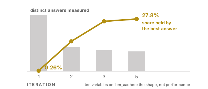
Convergence has a recognisable shape on a dashboard. Below is one of our own runs on the Hub, small enough to check by hand: ten variables, Miray on ibm_aachen, five iterations, 5,000 shots per iteration. It shows the shape rather than performance, because a ten-variable problem is solvable by enumeration.
| Iteration | Distinct bit strings measured | Share held by the best answer |
|---|---|---|
| 1 | 805 | 0.26% |
| 2 | 345 | 15.9% |
| 3 | 303 | 26.7% |
| 5 | 283 | 27.8% |
Iteration one is a haze: 5,000 shots came back as 805 distinct answers and the best one held 0.26 percent of them. By iteration five that same answer holds 27.8 percent, an amplification of about 107 times, and the number of distinct answers has fallen to 283. One bit string dominating the distribution is what convergence looks like here.
Two numbers are worth asking for whenever a run like this is presented. The found cost divided by the best-known cost, expressed in the objective's own units, since a quality figure normalised against anything else can be made to look arbitrarily good. And the quantum seconds actually consumed, summed per job, rather than the wall-clock time of the session around them.
Conclusion
Quantum optimization is a heuristic search engine for combinatorial decisions, and BF-DCQO is the version of it that fits today's hardware: no training loop, about ten iterations where a variational method needs around a hundred, a hundred times fewer total shots to the same target quality, and noise handling built into the update rule. On the hardest published benchmark it keeps pace with a 128-vCPU instance and with eight data-centre GPUs while drawing a million times fewer samples per second (Chandarana et al., arXiv:2603.13607), which is a trajectory worth watching rather than an advantage already delivered. The iteration count comes from the published experiments in arXiv:2409.04477.
The cheapest next step is to score a problem of your own against the triage above: count the decisions, count the interactions, and write down where the problem sits and what it would cost to run once. If it does not fit, that is a result worth having written down, and it is cheaper to reach here than in a pilot.
To run one instead, the hands-on Miray lab walks the dictionary above from formulation to ranked result on the free simulator, and the quantum portfolio optimization tutorial builds a cardinality-constrained selection problem with a genuine three-body risk term, which part two then scales past the simulator's qubit ceiling by decomposition. The Miray page covers the optimizer's scope, its interfaces and where it runs, Iskay covers the Qiskit Function route, and subscriptions live on the Hub marketplace. If you are looking for machine learning, session three, quantum machine learning, covers the evidence for Kipu's feature extraction. The full curriculum is available via the Academy page.