Educational disclaimer. Nothing here is complete or constitutes financial advice. Service names, endpoints and printed values are snapshots from the day this was written and will drift. Treat the live pages and the API references as the single source of truth.
1. Formulate
Build the HUBO dictionary by hand: return rewards, pairwise risk, a cardinality penalty, and one cubic term.
2. Run on Miray
Submit the dictionary to the free Miray simulator on the Kipu Quantum Hub and plot the risk/return frontier.
3. Judge the hardware
Approximate the gates a problem needs, price them against a chip's quality, and inform your expectations before you run on a QPU.
This lab runs in four phases: build the model (Steps 1 and 2), submit it (Step 3), check and read the answer (Steps 4 and 5), then evaluate wheter a QPU chip could solve it (Step 6). Every task below carries collapsed hints: Hint 1 tells you where you could look, Hint 2 gives additional pieces of the answer. Before you open any hint or solution: what do you think is happening here? Pause a minute on your own, or discuss with a partner. The solutions reveal the complete information that solves the problem.
Step 0: Set up the environment
Setup: uv project, SDK, credentials, CLI
You need a Python project folder, the Hub service SDK, and Hub credentials.
Build from scratch with uv
We teach with uv, use your favorite Python package manager at your own discretion. Either way, the code requires Python 3.11 or newer.
uv init kipu-optimization-lab
cd kipu-optimization-lab
uv venv
uv add qhub-service
Two later steps need one extra package each: a chart in Step 5, and an HTTP call in Step 6. Add them now or when you get there:
uv add matplotlib requests
The CLI is optional but recommended as a robust authorization route. It ships on npm and needs Node.js 20 or higher:
npm install -g @quantum-hub/qhubctl
After completion
To run the scripts in this lab:
uv run python task1_hubo.py
You can complete the whole formulation (Steps 1 and 2) of this lab locally and only need QHub credentials from Step 3 onward.
Step 1: Problem Formulation
Formulation is the most important step in solving an optimization problem on a quantum computer. Its size (number of variables), density (non-zero terms), and order (linear, quadratic, cubic, and so on) drive the circuit depth: the amount of sequential operations, or "length", of a quantum program. Current Quantum Processing Units are constrained in size (number of qubits) and error budget (hardware layout, qubit connectivity and 2-qubit-gate errors). Circuit depth is a decisive factor in whether a program runs inside a given QPU's error budget.
In this tutorial we will slip into the role of a financial analyst. While trading expected return against the risk of holding correlated pairs you pick 4 assets out of 8 fictional S&P 500 stocks. This problem is small, but structured enough to show the behaviour and to teach you how to scale it.
Create a file with the given data:
tickers = ["AAPL", "MSFT", "JPM", "XOM", "JNJ", "PG", "NVDA", "CVX"]
sector  = ["Tech", "Tech", "Financials", "Energy", "Health", "Staples", "Tech", "Energy"]

# Expected annual return, in percent (illustrative)
returns = [18.0, 16.0, 12.0, 11.0, 8.0, 7.0, 22.0, 10.0]

# High pairwise correlations: holding both concentrates risk
correlation = {
    (0, 1): 0.70,  # AAPL - MSFT   (mega-cap tech)
    (0, 6): 0.65,  # AAPL - NVDA
    (1, 6): 0.68,  # MSFT - NVDA
    (3, 7): 0.88,  # XOM  - CVX     (energy)
    (4, 5): 0.55,  # JNJ  - PG      (defensives)
}

k = 4   # hold exactly four names
Kipu's quantum optimizers minimize an objective written as a flat dictionary or array of variable interactions: a HUBO, the higher-order generalization of a QUBO. Each binary variable x_i is 1 if asset i is held, 0 if not. Three relationships go into the objective in this step:
- Reward return. A negative term
-return_ifor each asset, so the minimizer prefers holding high-return assets. - Penalize correlated pairs (risk). A positive quadratic (or higher) term on correlated pairs.
- Enforce the count. A cardinality penalty
(Σ x_i − k)²that is zero when exactly k assets are held.
Later we will assign weights for both risk and constraint penalties to balance their influence. Sometimes those values need to be rebalance.
Aside: the full objective, and how it becomes one HUBO dictionary
1. Add the terms. Summed together, the relationships above (plus the three-body term from Step 2) are a single objective the optimizer minimizes over the held/not-held vector x (each x_i ∈ {0, 1}):
H(x) = − Σ_i r_i x_i + λ Σ_{i<j} ρ_ij x_i x_j + Σ t_ijk x_i x_j x_k + P (Σ_i x_i − k)²
reading left to right: the return reward, the pairwise risk penalty, the three-body penalty, and the cardinality penalty, with return r_i, risk weight λ = risk_penalty, pairwise correlations ρ_ij, three-body penalty t, and cardinality weight P = card_penalty.
2. Flatten it to one dictionary. Kipu's optimizer does not take H(x) as algebra; it takes a flat dictionary keyed by the variable tuple each coefficient multiplies: () for the constant, (i,) for one variable, (i, j) for a pair, (i, j, k) for a triple. Three of the four terms already have that shape, return is linear (i,), pairwise risk is (i, j), the three-body term is (i, j, k), so they drop straight in.
3. Expand the one term that doesn't fit. (Σ x_i − k)² is a squared sum, not yet a sum of tuples. Expanding it (using x_i² = x_i for binary variables)
(Σ x_i − k)² = k² + (1 − 2k)·Σ x_i + 2·Σ_{i<j} x_i x_j
spreads it across three tuple types at once: a constant k², a linear part on every (i,), and a pairwise part on every (i, j). Those land on the same keys the return and risk terms already use, so the contributions add rather than replace.
Task 1. Fill in the three coefficients. Print the dictionary.
Start task1_hubo.py from this skeleton. The loops, the key syntax and the two weights are given. The coefficients are yours.
# task1_hubo.py
risk_penalty = 10.0    # weight on correlation risk
card_penalty = 50.0    # must dominate return + risk, see the encoding rule below
n = len(returns)

hubo = {}
hubo["()"] = ...                              # constant
for i in range(n):
    hubo[f"({i},)"] = ...                     # linear
for i in range(n):
    for j in range(i + 1, n):
        rho = correlation.get((i, j), 0.0)    # 0.0 for pairs not listed
        hubo[f"({i}, {j})"] = ...             # pairwise
The loops run over every pair, because the count penalty applies to all.
Hint 1, where to look
Part 3 of the aside above. Watch which keys the expansion lands on. Two of the three terms are already single pieces of the objective, listed individually:
- reward, linear:
− Σ_i r_i x_i - risk, quadratic:
λ Σ_{i<j} ρ_ij x_i x_j
The count penalty is not yet in that shape. It lands on the same keys once expanded, see Hint 2.
Hint 2, the three coefficients
Each key is a sum. The count penalty (Σ x_i − k)² must be expanded before it fits: (Σ x_i − k)² = k² + (1 − 2k)·Σ x_i + 2·Σ_{i<j} x_i x_j. Its three pieces, a constant, a linear part, and a pairwise part, land on the same keys as the reward and risk terms above, so they add onto them rather than replace them.
hubo["()"]           = card_penalty * k**2
hubo[f"({i},)"]      = -returns[i] + card_penalty * (1 - 2 * k)
hubo[f"({i}, {j})"]  = risk_penalty * rho + card_penalty * 2
Solution
# task1_hubo.py
risk_penalty = 10.0   # weight on correlation risk
card_penalty = 50.0   # must dominate return + risk so "exactly k" always wins
n = len(returns)

hubo = {"()": card_penalty * k**2}                      # constant term

for i, r in enumerate(returns):
    hubo[f"({i},)"] = -r + card_penalty * (1 - 2 * k)   # reward return, count term

for i in range(n):
    for j in range(i + 1, n):
        rho = correlation.get((i, j), 0.0)
        hubo[f"({i}, {j})"] = risk_penalty * rho + card_penalty * 2
The dictionary now has 1 constant, 8 linear and 28 pairwise keys.
Encoding rule. Keep the cardinality penalty roughly 10× larger than the return-plus-risk range. Too small and the optimizer "cheats" by holding three or five names to dodge a correlation penalty; too large and the correlation-risk signal is drowned out. The constraint and the objective have to stay in balance.
Step 2: Add the higher-order term
Everything in Step 1 is expressible as a QUBO: a pure means-and-pairwise-covariances model. During the 2008 financial crisis these pairwise models as we now know failed horribly. Means and pairwise covariances could not encode higher-order co-movement of multiple assets at all. Those models are computationally very expensive, and is the reason classical models are mostly pariwise-only. With quantum computers, we see the opportunity to encode the structure and eventually solve these problems buch better. Beware: the model is only as good as you formulate it!
BF-DCQO, the algorithm behind Kipu's optimizer, handles higher-order terms natively, with no quadratization and no auxiliary qubits, which is the subject of its own paper (arXiv:2409.04477). In dictionary terms it costs you exactly one more key.
Task 2. Add a 20.0 penalty on the AAPL, MSFT, NVDA triple. As tech assets they likely move together.
Hint 1, where to look
The tickers are indices 0, 1 and 6. One more key, one more index. Native higher-order solving: arXiv:2409.04477.
Hint 2, the shape of the answer
hubo["(0, 1, 6)"] = 20.0
Solution
# Higher-order term: holding ALL of AAPL, MSFT, NVDA together is worse
# than the three pairwise penalties suggest (joint-crash co-movement).
# A QUBO cannot represent this; a HUBO takes it as one more dictionary key.
hubo["(0, 1, 6)"] = 20.0
"All three assets moving together is a higher signal than the sum of all three pairs suggest". A degree-2 model and solver cannot encode that, so it either ignores the joint state or fakes it by quadratization. In practice that means: auxiliary variable, consistency penalties > more qubits and more depth.
Disclaimer: The pairwise-only model is what failed in 2008. While a cubic term lets you express joint co-movement,it does not make the model right. You chose the triple, the 20.0 and the correlations yourself, and the optimizer will faithfully return the best portfolio for the model you wrote. The model stays the binding limit.
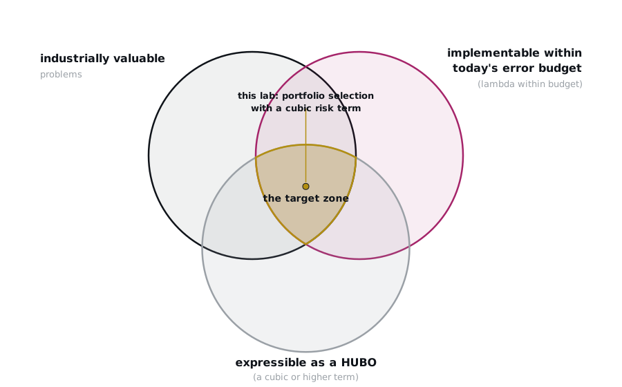
Koch, Panahiyan, Mukherjee, Doetsch (Lufthansa Industry Solutions) and Jaksch compared the HUBO-native route against the standard QUBO-penalty route on gate assignment, graph coloring and integer-programming instances, and measured at least 89.6 percent fewer CNOTs on every tested instance, with the flagship case a gate-assignment problem from an airport. The tech triple formulation from above stayed a native HUBO term; quadratizing the same term would have added an auxiliary variable plus consistency penalties and inflated the gate count. While not universal, the result is indicative and covers the three problem families above (arXiv:2511.17545, EPJ Quantum Technology 2026).
Optional: formulate with the Qiskit optimization mapper
Hand-building the dictionary is the best way to understand the encoding. On a large instance with many constraints you do not want to hand-expand (Σ x − k)² each time. Qiskit's modeling addon, qiskit-addon-opt-mapper, lets you state the problem declaratively and emits the HUBO for you (uv add qiskit-addon-opt-mapper):
from qiskit_addon_opt_mapper import OptimizationProblem
from qiskit_addon_opt_mapper.converters import OptimizationProblemToHubo

qp = OptimizationProblem(name="portfolio8")
x = [qp.binary_var(name=f"x{i}") for i in range(n)]

qp.minimize(
    linear={i: -returns[i] for i in range(n)},
    quadratic={(i, j): risk_penalty * rho for (i, j), rho in correlation.items()},
    higher_order={3: {(0, 1, 6): 20.0}},        # the cubic term, keyed by order
)
qp.linear_constraint(linear={i: 1 for i in range(n)}, sense="==", rhs=k, name="budget")

hubo_qp = OptimizationProblemToHubo(penalty=card_penalty).convert(qp)
The converter folds the equality constraint into the objective as the same squared penalty you built by hand, with penalty as its weight (None lets it pick one). Two conversion chores remain yours: the output keeps linear, quadratic and higher-order coefficients in separate accessors with tuple keys, so a short loop merges and stringifies them into Kipu's format, and the penalty expansion emits diagonal (i, i) entries that you fold into the linear (i,) terms first, since x·x = x for binary variables. It also reads docplex models and LP files, so an existing classical model comes across largely unchanged. For an example see Part 2.
Step 3: Run it on Miray
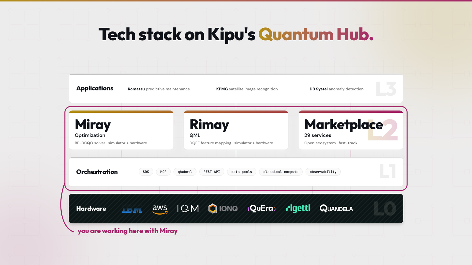
Miray is Kipu's Advanced Quantum Optimizer on the Kipu Quantum Hub, running the BF-DCQO engine (arXiv:2405.13898), with a free simulator tier and a one-line switch to hardware versions later.
What you need before submitting
SERVICE_ENDPOINTfor Miray Advanced Quantum Optimizer - Simulator. You obtain this by subscribing to the service. See using a service.ACCESS_KEY_IDandSECRET_ACCESS_KEY, the credential pair a subscription issues. See Qhub Service SDK.- Treat the keys like a password. An environment variable read with
os.getenvis the least-bad option; keep them out of scripts you want to upload or share with others. - You can delete and create new Application keys at any time in the Hub UI.
Reference pages for this step: Quickstart (account plus first run) and Service SDK (the client you are about to use).
Task 3. Submit the HUBO with 2000 shots, 6 iterations, 1 greedy pass. Print cost and solution.
Hint 1, where to look
Services have their own client, not the circuit provider: Service SDK. Create an Application and subscribe to Miray via the Marketplace. Check the documentation of the solver in the marketplace for details.
Hint 2, minimal setup
client = HubServiceClient(service_endpoint=..., access_key_id=..., secret_access_key=...)
execution = client.run(request={"problem": hubo, "problem_type": ..., "shots": ..., ...})
execution.wait_for_final_state()
print(execution.result())
problem is the dict we created earlier. problem_type is a string "binary" (0, 1), or "spin" (±1) for Ising-type problems. shots an int for the amout of shots per iteration, num_iterations int of iterations and num_greedy_passes int for post-processing and error correction. To use the HubServiceClient you need to install qhub.service.client (see Setup Step 0).
Solution
from qhub.service.client import HubServiceClient  # pip install qhub-service

client = HubServiceClient(
    service_endpoint=SERVICE_ENDPOINT,      # Miray Advanced Quantum Optimizer - Simulator
    access_key_id=ACCESS_KEY_ID,
    secret_access_key=SECRET_ACCESS_KEY,
)

execution = client.run(request={
    "problem": hubo,
    "problem_type": "binary",
    "shots": 2000,
    "num_iterations": 6,
    "num_greedy_passes": 1,
})
execution.wait_for_final_state()

response = execution.result()
print(response.result["cost"], response.result["mapped_solution"])
# Tip: increase shots and num_iterations for better results, or reduce for faster runtime.
This is the actual output from the verified run on the Miray Advanced Quantum Optimizer (Simulator), 2000 shots, 6 iterations, one greedy pass. Runtime: about 3 minutes.
cost = -56.5
mapped_solution = {0:1, 1:0, 2:1, 3:1, 4:0, 5:0, 6:1, 7:0}
A Hub service returns a result object, not just a bitstring. cost is the objective value the optimizer reached, mapped_solution is the held/not-held assignment keyed by your original asset index, and bitstring is the same solution in post-transpilation qubit order. Step 4 decodes it.
Optional: the same problem on Iskay via IBM Quantum
Iskay is the same optimizer delivered as a Qiskit Function on the IBM Quantum Platform. Same HUBO, different front door. If your stack is IBM, get in touch with your IBM Engagement Manager to get access.
from qiskit_ibm_catalog import QiskitFunctionsCatalog  # pip install qiskit-ibm-catalog

catalog = QiskitFunctionsCatalog(
    token=IBM_TOKEN, channel="ibm_quantum_platform", instance=INSTANCE_CRN,
)
iskay = catalog.load("kipu-quantum/iskay-quantum-optimizer")

job = iskay.run(
    problem=hubo,
    problem_type="binary",
    backend_name="ibm_fez",
    options={"shots": 2000, "num_iterations": 4},
)

result = job.result()
print(result["solution_info"]["cost"], result["solution"])
# Tip: increase shots and num_iterations for better results, or reduce for faster runtime.
Step 4: Decode and verify
4a. Comparison strategies
At this complexity, the chepest comparison strategy is greedy: sort by expected return, take the top four. NVDA is the highest earner at 22%, AAPL next at 18%, MSFT at 16%, JPM at 12%. Done.
4b. Check the result
For a problem at this size we can confirm the global optimum by brute force. But beware: complexity grows quickly; brute force stops being an option well before a realistic portfolio size. Here you can compare results with other classical (heuristic) solvers.
Task 4. Decode mapped_solution into the assets you hold. Does the greedy pick win here? And if it does not, how does it differ and why?
Hint 1, where to look
mapped_solution maps asset index to 0 or 1. You want the ones at 1. Greedy is one sort on returns, sliced to k.
greedy solution: sorted(range(n), key=lambda i: -returns[i])[:k]
Hint 2, the shape of the answer
Expect a key-type wrinkle: the mapped solution attribute shows integer keys with response.result["mapped_solution"]. Print solution and determine which assets the solver picked out of tickers[int(i)].
solution = response.result["mapped_solution"]
# selected = all tickers[i], where solution[i] == 1
Solution
solution = response.result["mapped_solution"]      # keys are string asset indices
selected = [tickers[int(i)] for i in solution if solution[i] == 1]
print(selected)
# -> ['AAPL', 'JPM', 'XOM', 'NVDA']

greedy = sorted(range(n), key=lambda i: -returns[i])[:k]
print([tickers[i] for i in sorted(greedy)])
# -> ['AAPL', 'MSFT', 'JPM', 'NVDA']
Three of the greedy four (AAPL, MSFT, NVDA) are exactly the penalized tech triple from Step 2. The naive pick maximizes headline return and concentrates risk in a single sector.
| Strategy | Holdings | Expected return | Cost | What happened |
|---|---|---|---|---|
| Naive (top-4 by return) | AAPL · MSFT · JPM · NVDA | 68% | −27.7 | holds the full tech triple |
| Quantum optimizer | AAPL · JPM · XOM · NVDA | 63% | −56.5 | diversified across 4 sectors |
Keeping the two highest-return tech bets (NVDA at 22%, AAPL at 18%) but dropping the third (MSFT, correlated 0.68 with NVDA and 0.70 with AAPL) in favor of JPM (financials) and XOM (energy) opens a 28.8-point gap in our model. The optimizer preserved its return appetite while keeping modelled risk low, giving up only 5 points of expected return for it.
Verification, given
energy(x) recomputes your own objective in plain Python, and the brute force enumerates all 256 assignments.
from itertools import product

def energy(x):
    e = card_penalty * k**2
    for i in range(n):
        e += (-returns[i] + card_penalty * (1 - 2 * k)) * x[i]
    for i in range(n):
        for j in range(i + 1, n):
            rho = correlation.get((i, j), 0.0)
            e += (risk_penalty * rho + card_penalty * 2) * x[i] * x[j]
    e += 20.0 * x[0] * x[1] * x[6]   # the three-body tech-triple term
    return e

x = tuple(solution[str(i)] for i in range(n))

assert sum(x) == k                                              # exactly k names held
assert abs(energy(x) - response.result["cost"]) < 1e-3          # cost is reproducible
best = min(product([0, 1], repeat=n), key=energy)               # brute force, 256 assignments
assert energy(best) == energy(x)                                # it is the global optimum
print("Verified: global optimum, exactly k held, energy consistent.")
Brute force arrives at the same energy −56.5 matching the quantum solver. It is only available to you because the problem is tiny. At 50 assets it would need to evaluate 10^15 assignments, and grows infeasibly large. On the other hand, the greedy method reads only the return, while the pairwise and cubic terms are where you modelled the concentration risk and priced that in.
Step 5: Plot the frontier
A single number ("cost −56.5") does not show why the pick is good. Plot every feasible portfolio in risk/return space and the answer is visual. There are only 70 ways to choose 4 of 8, so you can draw all of them.
This step needs matplotlib from Step 0.
Task 5. Write port_return(bits) and port_risk(bits) to plot your expected portfolio performance in a scatter plot.
Use this boilerplate for the scatter plot. Copy it, and add the scoring functions def port_return() and def port_risk().
import itertools
import matplotlib.pyplot as plt

GOLD, AMARANTH, BG, FG = "#b38f12", "#a52469", "#FFFFFF", "#0f1319"

# Complete these two functions (Task 5) before running the cell:
# with the `...` stubs in place the plot below raises a TypeError.
def port_return(bits):
    ...        # Task 5

def port_risk(bits):
    ...        # Task 5

pts = [(port_risk(b), port_return(b)) for b in
       ([1 if i in c else 0 for i in range(n)]
        for c in itertools.combinations(range(n), k))]

quantum = [1, 0, 1, 1, 0, 0, 1, 0]                          # your verified solution
gcombo  = sorted(range(n), key=lambda i: -returns[i])[:k]
greedy  = [1 if i in gcombo else 0 for i in range(n)]

fig, ax = plt.subplots(figsize=(7, 5))
fig.patch.set_facecolor(BG); ax.set_facecolor(BG)
ax.scatter([p[0] for p in pts], [p[1] for p in pts], c="#cfcdcd", s=30, label="all portfolios")
ax.scatter(port_risk(quantum), port_return(quantum), c=GOLD, s=190, edgecolors="white", lw=1.5, zorder=3, label="Kipu quantum optimum")
ax.scatter(port_risk(greedy), port_return(greedy), facecolors="none", edgecolors=GOLD, s=190, lw=2.4, zorder=2, label="naive (top-4 return)")
ax.set_xlabel("Correlation risk score (lower is safer)", color=FG)
ax.set_ylabel("Expected return (%)", color=FG)
for sp in ("top", "right"): ax.spines[sp].set_visible(False)
ax.legend(frameon=False)
plt.show()
Hint 1, where to look
Return: is the sum(returns[i]) of all picked assets
Risk: is the sum(rho for (i, j), rho in correlation.items()) for all picked assets i and j; PLUS the HUBO risk term if bits[0] and bits[1] and bits[6] are picked.
Hint 2, the shape of the answer
def port_return(bits): return sum(returns[i] for i in range(n) if bits[i])

def port_risk(bits):
    r = sum(rho for (i, j), rho in correlation.items() if bits[i] and bits[j])
    if bits[0] and bits[1] and bits[6]:
        r += 20.0 / risk_penalty            # three-body term, normalized risk scale
port_risk sums rho over correlation.items() where both ends are held, then adds 20.0 / risk_penalty if indices 0, 1 and 6 are all held.
Solution
import itertools
import matplotlib.pyplot as plt

# Kipu brand colors (tokens.css)
GOLD, AMARANTH, BG, FG = "#b38f12", "#a52469", "#FFFFFF", "#0f1319"

def port_return(bits):
    return sum(returns[i] for i in range(n) if bits[i])

def port_risk(bits):
    r = sum(rho for (i, j), rho in correlation.items() if bits[i] and bits[j])
    if bits[0] and bits[1] and bits[6]:
        r += 20.0 / risk_penalty
    return r

pts = []
for combo in itertools.combinations(range(n), k):
    bits = [1 if i in combo else 0 for i in range(n)]
    pts.append((port_risk(bits), port_return(bits)))

quantum = [1, 0, 1, 1, 0, 0, 1, 0]                          # verified solution
gcombo  = sorted(range(n), key=lambda i: -returns[i])[:k]   # naive pick
greedy  = [1 if i in gcombo else 0 for i in range(n)]

fig, ax = plt.subplots(figsize=(7, 5))
fig.patch.set_facecolor(BG); ax.set_facecolor(BG)
ax.scatter([p[0] for p in pts], [p[1] for p in pts], c="#cfcdcd", s=30, label="all portfolios")
ax.scatter(port_risk(quantum), port_return(quantum), c=GOLD, s=190, edgecolors="white", lw=1.5, zorder=3, label="Kipu quantum optimum")
ax.scatter(port_risk(greedy),  port_return(greedy),  facecolors="none", edgecolors=GOLD, s=190, lw=2.4, zorder=2, label="naive (top-4 return)")
ax.set_xlabel("Correlation risk score (lower is safer)", color=FG)
ax.set_ylabel("Expected return (%)", color=FG)
ax.set_title("4-of-8 portfolios: risk vs return", color=FG, fontweight="bold", loc="left")
for s in ("top", "right"): ax.spines[s].set_visible(False)
ax.legend(frameon=False)
plt.show()
The verified optimum trades little return for much reduced risk:
| Risk | Return | Portfolio | Role |
|---|---|---|---|
| 0.65 | 63 | AAPL / JPM / XOM / NVDA | quantum optimum (verified) |
| 4.03 | 68 | AAPL / MSFT / JPM / NVDA | naive pick (max-return) |
An honest reading of that chart is more nuanced. The naive pick is not irrational: it sits on the efficiency frontier, at the maximum-return corner. It takes on large risk for the last bit of return. Going from the quantum optimum to the naive pick buys +5 points of return for +3.4 points of risk, while the step into the optimum bought +10 return for +0.65 risk. The risk appetite you encoded (risk_penalty = 10) controls where the optimizer lands and can be tuned. It is a modeling choice.
Step 6: Will it run on hardware?
Everything so far ran on a simulator, and a simulator has no chip: no error rates, no wiring, no clock. Point the same dictionary at hardware and the question becomes whether your problem and the machine line up.
Three properties of your problem meet three properties of the hardware. Call it the 3 + 3.
| Your problem | has to fit | The chip |
|---|---|---|
| variables, how many yes/no decisions | inside | qubits, a hard ceiling |
| density, how many interactions you wrote | inside | error budget, roughly 1 / error per gate |
| order, how many variables per term | inside | layout, how the qubits are wired together |
The rows are not independent, which is the whole subtlety. Density and order both inflate the gate count, and the layout decides how much extra you pay to deliver those gates, so the bottom two rows meet in one number. Only the top row is a clean ceiling: 8 variables need 8 qubits, and every chip in the Hub list has hundreds.
That is why qubit count is the least interesting number on a spec sheet at these sizes: a sparse model with many variables can run where a dense model with far fewer variables fails, because interactions, not variables, drive the gate count.
Three quantities turn the bottom two rows into arithmetic.
1. What your model demands. Every interaction in your dictionary becomes two-qubit gates. A d-body term costs 2(d − 1) of them, so each pair costs 2 and your tech triple costs 4. Sum over the dictionary and you have the gate count your model asks for, before any chip has a say.
2. What the chip charges to deliver it. Two variables can only interact if their qubits are physically wired together. When they are not, the compiler shuttles them toward each other, and every move is more two-qubit gates. The wiring pattern therefore multiplies your gate count:
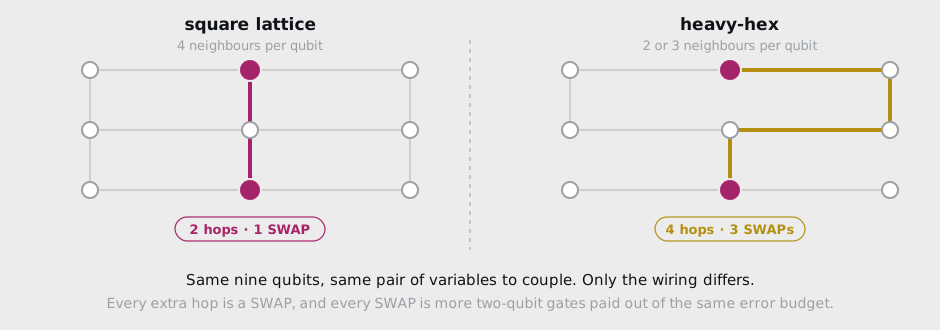
Two chips with identical gate quality can differ by a large factor purely from how they are wired. Whatever that factor is for your problem, you learn it by transpiling, not by looking it up: routing cost depends on your model's density as much as on the lattice, and a sparse model on heavy-hex can beat a dense one on a grid.
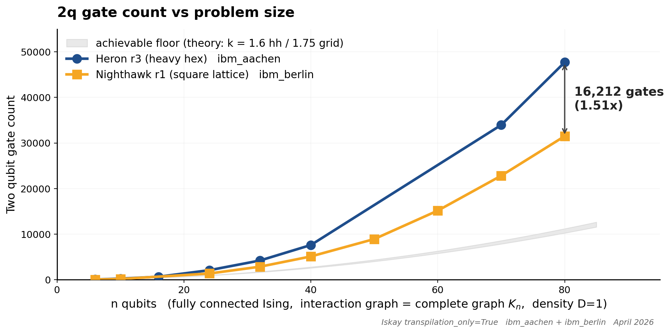
That factor is not hypothetical: transpiling the same fully connected Ising problem (Iskay, transpilation-only, no QPU time spent) onto ibm_aachen (Heron r3, heavy-hex) and ibm_berlin (Nighthawk r1, square lattice) in April 2026 shows it growing with problem size, reaching a roughly 1.51 times advantage in lower two-qubit gate count compared to current heavy-hex at n = 80.
3. What the chip gets wrong. Every two-qubit gate has a failure probability, published per chip and refreshed daily in its calibration data.
Put the three together and you have one number:
λ  =  N_2q × r × p_2q  +  n × p_readout  +  decoherence

N_2q       two-qubit gates your model needs, summed as 2(d − 1) per d-body term
r          routing factor of the wiring, measured by transpiling, not looked up
p_2q       error per two-qubit gate, from the chip's live calibration
p_readout  error per measurement; every shot reads out all n qubits once
λ is the accumulated error of one run, every channel added. On today's chips the two-qubit term dominates once the model has any size, readout matters most for small dense-readout problems, and the decoherence share depends on idle time the transpiler sets, so it is named here and measured by transpiling.
Task 6 computes this with the routing factor left at one. That gives you a floor, not a forecast: a real chip can only be worse, and how much worse is a transpiler question rather than a lookup.
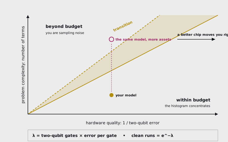
λ is the expected number of errors in a single run, so the fraction of runs that come back clean is
P(clean) = e^(−λ) λ = 1 → 37% λ = 3 → 5% λ = 5 → under 1%
and only clean runs teach the optimizer anything. Small λ and the histogram concentrates on one answer, which is what convergence looks like from the outside. Large λ and you are sampling noise: you may still stumble onto the optimum, but you will have no way to tell that you did.
Both quantities live on one picture, and it is the picture worth carrying out of this lab:
Read it in three moves. Your model's gate count sets your height, so every modelling choice (fewer variables, sparser couplings, lower degree) moves you down toward safety. The chip's quality sets your horizontal position, so a better chip moves you right and can handle a taller model. Whichever side of the band you sit on tells you what to do next: run it, lean on post-processing, or reshape the model.
The same split is how to read a hardware roadmap. Improvement is k_total = k_error × k_architecture: better gates and better wiring are separate levers, and the wiring lever is measured for your problem rather than quoted from a spec sheet.
This λ is the number you will defend when you ask for real QPU budget on a problem, so learn to get it before you spend.
Task 6. Choose 2+ available hardware QPUs from the Kipu Quantum Hub. Check the recent calibration data for the median two qubit fidelity and compare.
Hint 1, where to look
Backends are listed publicly at Hub quantum backends, ids in the form ibm.qpu.boston. Calibration can be retreived from the UI, from the SDK or as an API request via /quantum/backends/{id}/calibration, using your Hub personal access token in an X-Auth-Token header. Error per gate is 1 − fidelity.
Hint 2, the structure
cal = requests.get(f"{API}/{chip}/calibration", headers={"X-Auth-Token": TOKEN}).json()
p_2q = 1 - cal["median_two_qubit_fidelity"]["value"]     # also: median_t1, median_t2
Solution
import math, os, requests

TOKEN = os.environ["KQH_PERSONAL_ACCESS_TOKEN"]
API = "https://api.hub.kipu-quantum.com/quantum/backends"

def error_per_gate(backend_id):
    cal = requests.get(f"{API}/{backend_id}/calibration",
                       headers={"X-Auth-Token": TOKEN}, timeout=30).json()
    return 1 - cal["median_two_qubit_fidelity"]["value"], cal["calibrated_at"]

def degree(key):
    if key == "()":
        return 0
    return key.count(",") if key.endswith(",)") else key.count(",") + 1

def gates_needed(hubo):
    # a d-body term costs 2(d-1) two-qubit gates; constants and linear terms cost none
    return sum(2 * (degree(key) - 1) for key in hubo if degree(key) >= 2)

n_gates = gates_needed(hubo)
for chip in ("ibm.qpu.boston", "ibm.qpu.marrakesh"):
    p, when = error_per_gate(chip)
    lam = n_gates * p
    print(f"{chip:20} p_2q={p:.1e}  lambda={lam:.3f}  clean={math.exp(-lam):.0%}  (cal {when[:10]})")
To estimate gate count: for each term in the dictionary add
2(d − 1)for every key of degreed=2or higher. Thenλ = N_2q * p_2q, ignoring routing for now.
The porfolio hubo sits at minimum 60 two-qubit gates: 28 pairs at 2 each, plus the triple at 4. Against calibration from 24 August 2026, and before any routing overhead and asusming a perfect gate set:
| Chip | Gates (est.) | Error per gate | lambda | Runs coming back clean |
|---|---|---|---|---|
ibm.qpu.boston | 60 | 1.4e-3 | 0.08 | ~92% |
ibm.qpu.marrakesh | 60 | 3.4e-3 | 0.20 | ~82% |
Both sit comfortably below lambda < 2, which is expected for an 8-variable problem: it fits anywhere, and the QPU chip barely matters. When the model grows, and more terms are added, lambda increses rapidly. A fully connected quadratic model has n(n−1)/2 pairs:
| Assets | Pairs | Gates | lambda on ibm.qpu-boston | Verdict |
|---|---|---|---|---|
| 8 | 28 | 60 | 0.08 | concentrates |
| 50 | 1,225 | 2,450 | ~3.4 | marginal, post-processing required |
| 250 | 31,125 | 62,250 | ~87 | out of reach, reshape or decompose |
Density, not variable count, is the important factor driving the gate count. To get around that limitation Part 2 introduces a decomposition technique for large problems. It cuts them up into hardware-sized pieces instead.
Caution: the calculation above assumes perfect connectivity (all-to-all) and a perfect gate sets. Actual circuits might be 4+ times larger once you account for routing and chip specifics. Transpilation_only runs can help estimate complexity and return the circuit information without submitting a job to the backend.
The definition, extended
The business lesson gives the first two senses. Having formulated a HUBO, submitted it and verified what came back, the third is yours.
quan·tum op·ti·mi·za·tion
/ˈkwɒn.təm ˌɒp.tɪmaɪˈzeɪ.ʃən/noun
- 1
act or process of finding the absolute highest or lowest values of a function under specific rules.
- 2
a method that maps complex math problems into quantum states, using phenomena like superposition and tunneling to navigate tricky solution landscapes.
- 3
Kipu Optimizers solve HUBOs as a service on the Kipu Quantum Hub. You can subscribe to the solver and build the wrapper with your domain-specific knowledge around it.
Documentation: Kipu Quantum Hub | Hub docs | Quickstart | Service SDK | Using a service | Access tokens | Iskay on IBM Quantum | Kipu Quantum Academy
Research: BF-DCQO, the optimizer's algorithm (arXiv:2405.13898) | BF-DCQO for higher-order (HUBO) optimization (arXiv:2409.04477) | DCQO portfolio optimization on IonQ, 20 assets (arXiv:2308.15475) | Large-scale portfolio optimization on a trapped-ion quantum computer (arXiv:2602.23976)