Superposition and Entanglement
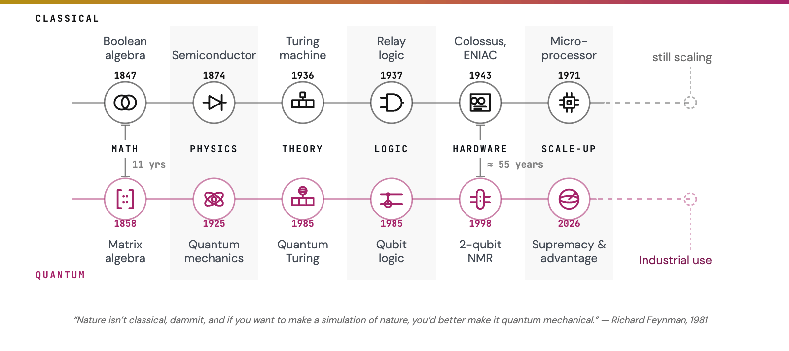
If you have followed the Kipu Quantum Hub Quickstart Guide, you have already run your first quantum job. In addition to the classical standard logic set with the not gate (turning a 0 into a 1), and/or gates, quantum computing introduces additional, probabilistic and connecting operations to our computational toolset. However those operations are short-lived. Qubits are highly unstable and once we measure them to get our solution, we measure the statistics of multiple experiments (in the following we will call them shots). That means current quantum algorithms need to be hand-crafted based on the problem and hardware specification. A common misconception is that quantum computing is weird and not even the brightest minds in physics understand it. As we will discover, the origins of quantum and classical computing have been studied for centuries and show surprising parallels.
Because quantum bits (qubits) are based on the so-called Hilbert space, they add probabilistic states in between 0 and 1. A famous example is the Hadamard Gate H: it introduces a state that is equidistant to 0 and 1, thus producing a state with equally distributed 50/50 statistics. To get an intuition about single qubit gates, play around with the Bloch Sphere Demo by James Weaver and Ismael Faro Sertage. What happens if you press the H button?
Working with superpositions, such as the single H-Gate operation, makes quantum computers inherently probabilistic. An effect you know from everyday life, like flipping a coin. Industries like finance, insurance and weather forecasters have built entire professions around understanding probabilistic data and getting "lucky" more often than not. In addition to probability (superposition), we can connect (entangle) outcomes. That means one result will depend on the other, without knowing either one of them in advance. Think two connected coins that always land both on heads, or both on tails. Under the hood these properties give quantum computers their strength. See this as an invitation to develop an effective mental model of quantum computing that makes it stochastic, yet deterministic and fully predictable. Let us start from the beginning.
Both modalities are well studied and their concepts originate from ideas that are over 2000 years old. Due to its unstable and miniature nature, quantum milestones now trail around 50 years behind their classical counterparts. To fulfill the potential and eventual societal change quantum can bring, specialists from all professions need to get involved. Just like you right now, completing the tutorials. From the Kipu team, a big ♥-thank you for your commitment and efforts that make that future a little brighter.
About our approach
The rules below govern the hands-on tutorial this primer belongs to.
Following scientific consensus, this tutorial consists of sub-tasks with short breaks to reflect before revealing the answer. Six of the seven steps will have you write a small Python file and run it from a terminal, so you finish with a directory you can come back to. The seventh and last step is a mental map using the Kipu Quantum Hub as a tool on your quantum journey.
A note about hints in this course
Under some tasks you might find collapsed hints that will help you get to an answer. Before using them, take a short breather and think about what you expect. If you have a partner or colleague, or even a favorite LLM model, discuss with them.
Hints follow a structure:
- Hint 1, where to look. Points at the docs page or a local command that might help you surface the answer. No direct answers here.
- Hint 2, the shape of the answer. Describes the structure of what you are reaching for without naming it. Enough to unstick you, not enough to skip the thinking.
- Solution. The full working code, verified against the live Hub, with a copy button.
Opening the Solution first is the one reliable way to get nothing out of this page. Ideally, we build the right frameworks for you to find the answer in the reference and systematically solve the problem in front of you. In the end, that skill is what will make you independent of tutorials like this one.
Your move
Done with the tutorial? Here is where to take it.
- Scale the circuit. Take the same idea to three qubits and correlate all three. Predict which outcomes survive before you run it, same discipline as Step 3b.
- Change the backend. Rerun
task4_run.pyagainstazure.ionq.simulator, the other free backend, and see whether the shape holds. Different vendor, different gate set, same physics. - Read your own transpilation. Print
transpiled.draw()next tocircuit.draw()and work out what the compiler did to your circuit and why. That gap is where circuit depth, and therefore hardware feasibility, actually comes from. - Find where the tools stop. Run
qhubctl login, thenqhubctl list-contextsandqhubctl services list. Then note the gap: there is no CLI command for listing backends, submitting a raw quantum job, or inspecting one. That surface exists only in the SDK, the dashboard and MCP. Knowing where a tool stops is worth as much as knowing what it does. - Do something with an optimizer. You now have a working credential and a working harness. The quantum portfolio optimization tutorial is the natural next step, and it runs at L2 on the free Miray simulator.
- Bring your problem. If you have a candidate application and want to assess practical fit on current hardware, the Kipu Quantum Academy is built for that.
Documentation: Kipu Quantum Hub | Hub docs | Quickstart | Quantum SDK reference | Access tokens | Managing quantum jobs | CLI reference | MCP server setup | Backends catalogue | Dashboard
Ready for the hands-on part? Start the hands-on tutorial.